Supercontinuum in a photonic crystal fibre#

The canonical solid-core supercontinuum: a 50 fs, 10 kW sech pulse at 835 nm in 15 cm of photonic crystal fibre, pumped in anomalous dispersion close to the zero-dispersion wavelength. The parameters are those of Fig. 3 of the review by Dudley, Genty and Coen, the standard test of a generalised nonlinear Schrödinger equation solver: the fibre’s dispersion as ten Taylor coefficients about the pump (beta_2 to beta_10), gamma = 0.11 /W/m, self-steepening, and silica’s Raman response.

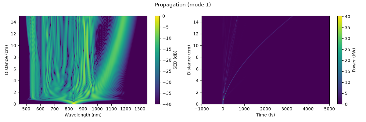
The launch is a soliton of order N = 8.7. It compresses within the first centimetre and then breaks up (soliton fission) into fundamental solitons, which shift to longer wavelengths by the Raman effect, and dispersive waves phase-matched to them on the short-wavelength side of the zero-dispersion wavelength.

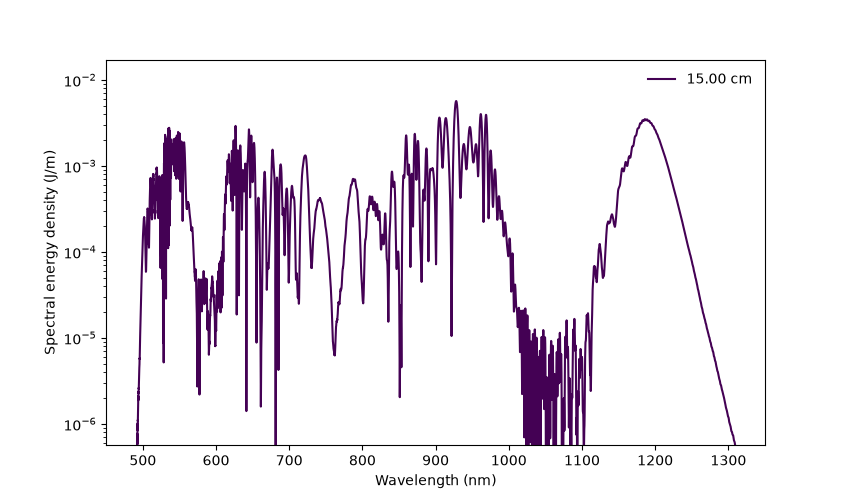
What to look for. In the spectral map the continuum spreads to both sides at fission, near 1 cm; the red-shifting solitons then curve away to beyond 1200 nm and the dispersive waves gather near 500-600 nm. In the time domain the solitons, slowed as they shift, walk off to positive delay.

What is approximate. The fibre is described by its dispersion and gamma at the pump alone, as in the review: no wavelength dependence of the effective area beyond self-steepening’s. One seeded shot of input noise is propagated; the shot-to-shot coherence the review studies with ensembles is not estimated here.

Recipe.example("fibre_supercontinuum") is this run as a recipe.

Reference: J. M. Dudley, G. Genty and S. Coen, Supercontinuum generation in photonic crystal fiber, Rev. Mod. Phys. 78, 1135-1184 (2006), section III and Fig. 3.

The run#

The Taylor coefficients are in s^n/m, about 835 nm. The 12.5 ps window holds the solitons as they walk off; 201 planes resolve the evolution along the fibre.

import time

from solprop.driver import prop_gnlse
from solprop.plotting import prop_2d, spec_1d

started = time.perf_counter()
output = prop_gnlse(
    0.11,
    0.15,
    [
        0.0,
        0.0,
        -11.830e-27,
        8.1038e-41,
        -9.5205e-56,
        2.0737e-70,
        -5.3943e-85,
        1.3486e-99,
        -2.5495e-114,
        3.0524e-129,
        -1.7140e-144,
    ],
    wavelength=835e-9,
    wavelength_limits=(400e-9, 2e-6),
    trange=12.5e-12,
    fwhm=50e-15,
    shape="sech",
    peak_power=10e3,
    raman=True,
    shock=True,
    n_save=201,
    seed=20261106,
    progress="none",
)
print(f"Propagated in {time.perf_counter() - started:.1f} s")

Propagated in 22.4 s

The evolution along the fibre#

The spectral energy density in decibels beside the instantaneous power, against distance, as in the review’s figure.

prop_2d(
    output,
    "wavelength",
    spec_range=(450e-9, 1350e-9),
    time_range=(-1e-12, 5e-12),
    db_min=-40.0,
)

[<Figure size 1200x400 with 4 Axes>]

The spectrum at the exit#

spec_1d(output, 0.15, "wavelength", spec_range=(450e-9, 1350e-9), log_min=1e-4)

<Figure size 850x500 with 1 Axes>

Supercontinuum in a photonic crystal fibre#

The run#

The evolution along the fibre#

The spectrum at the exit#

Related reading#