A pulse in two channels of a graded-index fibre

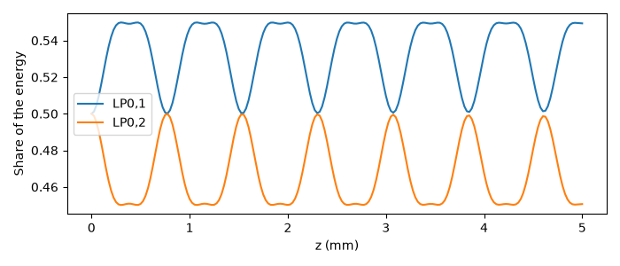
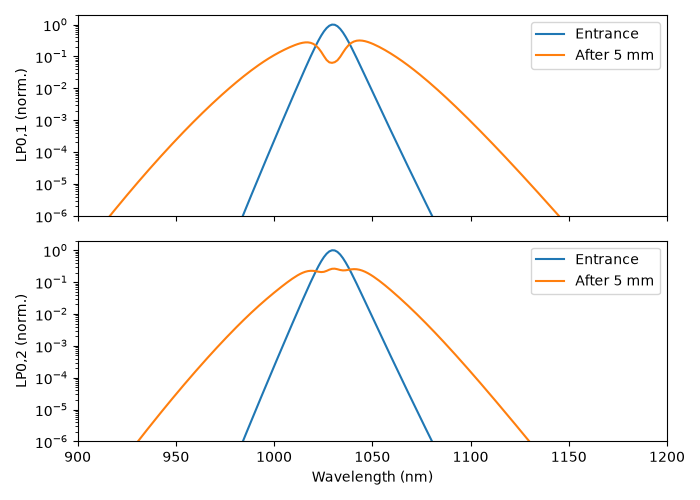
A parabolic graded-index core has channels whose group delays nearly agree, which is what the profile is for. This example launches a femtosecond pulse equally into the two lowest radial LP channels of a 25 um core and follows it for 5 mm with the core’s Kerr response. The channels broaden, and the Kerr term moves energy between them as their relative phase turns.

on_grid() takes the guide’s frequency knots and node rule from the run’s grid, so the setup can be held as a recipe: Recipe.example("graded_index_fibre") is this run. The material is a constant index, so all the dispersion here is the guide’s. The channel count, element count and knots are the numerical choices to refine, as the self-imaging example explains.

import matplotlib.pyplot as plt
import numpy as np

from solprop.constants import C
from solprop.driver import Simulation
from solprop.grid import FieldGrid
from solprop.modes import (
    GradedIndexProvider,
    IndexMaterial,
    MaterialKerr,
    ModalGuide,
    PowerLawPermittivity,
)
from solprop.processing import grid_of

RADIUS = 25e-6
"""Core radius, m."""

CONTRAST = 0.005
"""Index contrast Delta, dimensionless: eps = eps_axis (1 - 2 Delta rho^2)."""

AXIS_INDEX = 1.45
"""Index on the axis."""

N2 = 2.6e-20
"""Nonlinear index of the core, m^2/W, a typical silica value at the pump."""

WAVELENGTH = 1.03e-6
"""Pump wavelength, m."""

'Pump wavelength, m.'

The guide. The LP family is the scalar weak-guidance approximation, and the core carries the only response: the exterior is linear.

provider = GradedIndexProvider(
    permittivity=PowerLawPermittivity(IndexMaterial(AXIS_INDEX), CONTRAST),
    exterior=IndexMaterial(AXIS_INDEX * np.sqrt(1.0 - 2.0 * CONTRAST)),
    radius=RADIUS,
    family="LP",
    count=2,
    elements=64,
    extent=2.0,
    core_responses=(MaterialKerr(n2=N2, at=WAVELENGTH),),
)

The grid, then the guide on it. The count of knots depends on the band: on this one, 13 and 17 leave the interpolated basis further from orthonormal at the long-wavelength end than the route calls the identity, and it warns by name; 21 does not.

grid = FieldGrid.from_limits(0.005, WAVELENGTH, (0.9e-6, 1.2e-6), 2e-12)
guide = ModalGuide.on_grid(grid, provider, knots=21, n_r=2)
labels = [label.display_label for label in guide.mode_collection.channel_labels]
print(labels)

['LP0,1', 'LP0,2']

A 100 fs pulse, shared equally between the two channels. The saved planes are close enough to resolve the beat below: at one plane per millimetre it would alias.

simulation = Simulation.from_waveguide(
    (),
    0.005,
    provider=guide,
    grid=grid,
    wavelength=WAVELENGTH,
    fwhm=100e-15,
    energy=100e-9,
    shape="sech",
    launch={labels[0]: 0.5, labels[1]: 0.5},
    n_save=201,
    rtol=1e-5,
    noise=None,
    absorber=False,
    boundary_check=None,
)
output = simulation.run(progress="none")

The share of the energy in each channel along the fibre. The Kerr term couples the channels, so the shares move, while their sum stays that of the launch to the run’s tolerance. They beat with the channels’ relative phase: the period is close to 2 pi / Delta beta, with Delta beta from the parabolic closed form of the self-imaging example.

saved = grid_of(output)
active = saved.omega > 0
order = np.argsort(2 * np.pi * C / saved.omega[active])
wavelength = (2 * np.pi * C / saved.omega[active])[order]
spectra = np.abs(output.fields("fft")[:, :, 0, active][..., order]) ** 2
energy_in_channel = np.sum(spectra, axis=-1)
total = np.sum(energy_in_channel, axis=1)
print(f"total energy changed by {abs(total[-1] / total[0] - 1):.1e}")
q = 2 * np.pi / WAVELENGTH * RADIUS * AXIS_INDEX
ideal = np.sqrt(q * q - 2 * q * np.sqrt(2 * CONTRAST) * np.array([1, 3])) / RADIUS
print(f"closed-form beat length {2 * np.pi / (ideal[0] - ideal[1]) * 1e3:.3f} mm")
figure, axis = plt.subplots(figsize=(7, 3))
z = np.asarray(output["z"])
for index, label in enumerate(labels):
    axis.plot(z * 1e3, energy_in_channel[:, index] / total, label=label)
axis.set(xlabel="z (mm)", ylabel="Share of the energy")
axis.legend()
figure.tight_layout()

total energy changed by 3.6e-08
closed-form beat length 0.785 mm

The spectrum of each channel at the entrance and the exit, on one scale for each channel.

figure, axes = plt.subplots(2, 1, figsize=(7, 5), sharex=True)
for index, axis in enumerate(axes):
    peak = np.max(spectra[0, index])
    axis.semilogy(wavelength * 1e9, spectra[0, index] / peak, label="Entrance")
    axis.semilogy(wavelength * 1e9, spectra[-1, index] / peak, label="After 5 mm")
    axis.set(ylabel=f"{labels[index]} (norm.)", ylim=(1e-6, 2), xlim=(900, 1200))
    axis.legend()
axes[-1].set(xlabel="Wavelength (nm)")
figure.tight_layout()

plt.show()